

Attempt the next – ask any Excel person for his/ her favorite Excel formulation. Most of the time, you’ll hear simply this one title -VLOOKUP. And this fame is for all the proper causes. From finance groups reconciling numbers to analysts cleansing messy datasets, this operate quietly powers probably the most essential operations in a spreadsheet. So, sure, if you don’t already, you need to know all about VLOOKUP.
And if this significance is evident to you, and you’re studying this text to be taught VLOOKUP, kudos! You might be on the proper place, as right here, we will discover all there may be to find out about VLOOKUP, the way it works, and what all you are able to do with it. The most effective half – we are going to undergo this studying expertise with actual examples.
So, comply with alongside, and be a grasp of VLOOKUP very quickly.
What’s VLOOKUP?
First issues first. What does “VLOOKUP” even imply? The title comes from a easy logic it follows – Vertical Lookup. In essence, it’s an Excel operate that searches for a worth, as indicated by the “lookup” moniker. But it surely does so in a really particular method.
It appears to be like for the worth within the first column of a desk and returns a corresponding worth from one other column in the identical row. The operate works vertically (prime to backside), which is the place the title comes from.
Consider it as Excel’s means of claiming: “Discover this merchandise, then carry me the element related to it.”
In easy phrases, VLOOKUP helps you:
- Match information between two tables
- Retrieve associated info immediately
- Eradicate guide looking out and copy-pasting
- Scale back errors in repetitive information duties
Here’s a take a look at its significance intimately.
Additionally learn: Microsoft Excel for Information Evaluation
How VLOOKUP Helps
We all know now that at its core, VLOOKUP solves one of the frequent issues in information work: discovering the proper worth in seconds. For instance, if in case you have an inventory of product names and costs, VLOOKUP can rapidly discover the value of a particular product with out you manually scanning the desk.
Now merely think about this checklist scaled 1000 instances.
As a result of that’s the type of information quantity that large firms work with. A number of spreadsheets home information factors in hundreds, and manually sifting via such information is like discovering a needle in a haystack.
That is the place VLOOKUP shines. Regardless of the amount of the information, VLOOKUP will work simply as tremendous throughout gigantic spreadsheets too. In such eventualities, whether or not you’re matching product costs or IDs, merging experiences, or constructing dashboards, it’s simple to see how mastering VLOOKUP can save hours of guide effort.
Listed below are some real-life use instances the place VLOOKUP is used each day:
- Fetching product costs from a grasp pricing sheet
- Matching buyer IDs with names, emails, or buy historical past
- Pulling worker particulars (division, function, wage band) from HR databases
- Mapping order IDs to order standing in operations experiences
- Merging gross sales information from a number of regional spreadsheets into one report
- Retrieving stock ranges for particular SKUs from warehouse data
- Linking bill numbers to fee standing in finance trackers
and the checklist goes on. Hopefully, this offers youa. gist of simply how necessary VLOOKUP can show to be. Now that the requirement is evident, let’s transfer on to really understanding the operate.
Understanding VLOOKUP
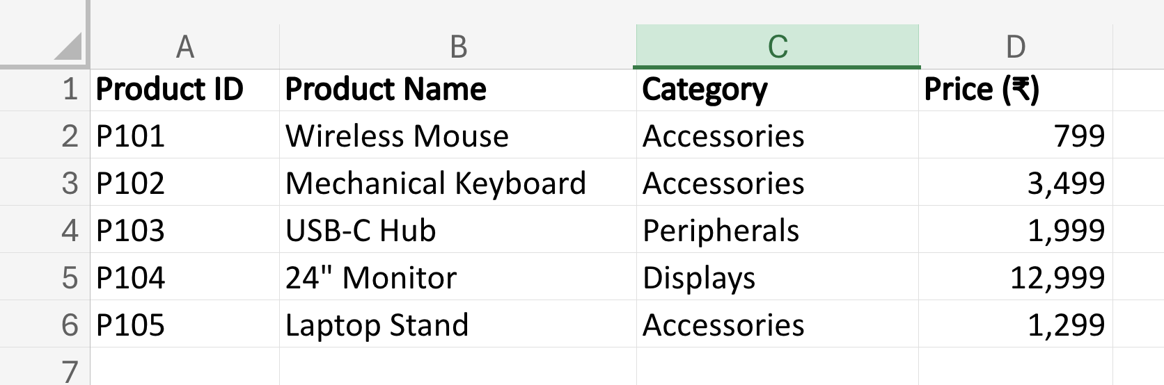
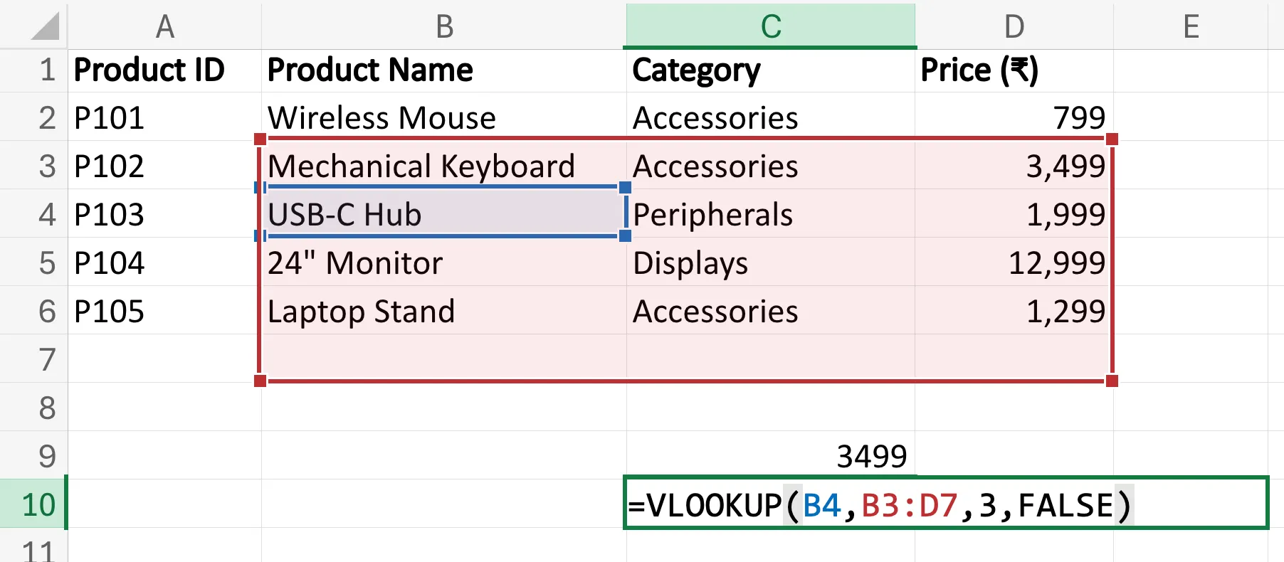
Allow us to attempt to perceive VLOOKUP with an instance. Contemplate the information within the screenshot beneath. It lists the merchandise in an IT warehouse, together with their product IDs and related prices. I’ve saved this checklist brief for utmost readability in understanding the operate.
Now, think about you want to discover the value of the Mechanical Keyboard from this checklist. Right here is the VLOOKUP formulation for a similar:
=VLOOKUP(B3,B2:D6,3,FALSE)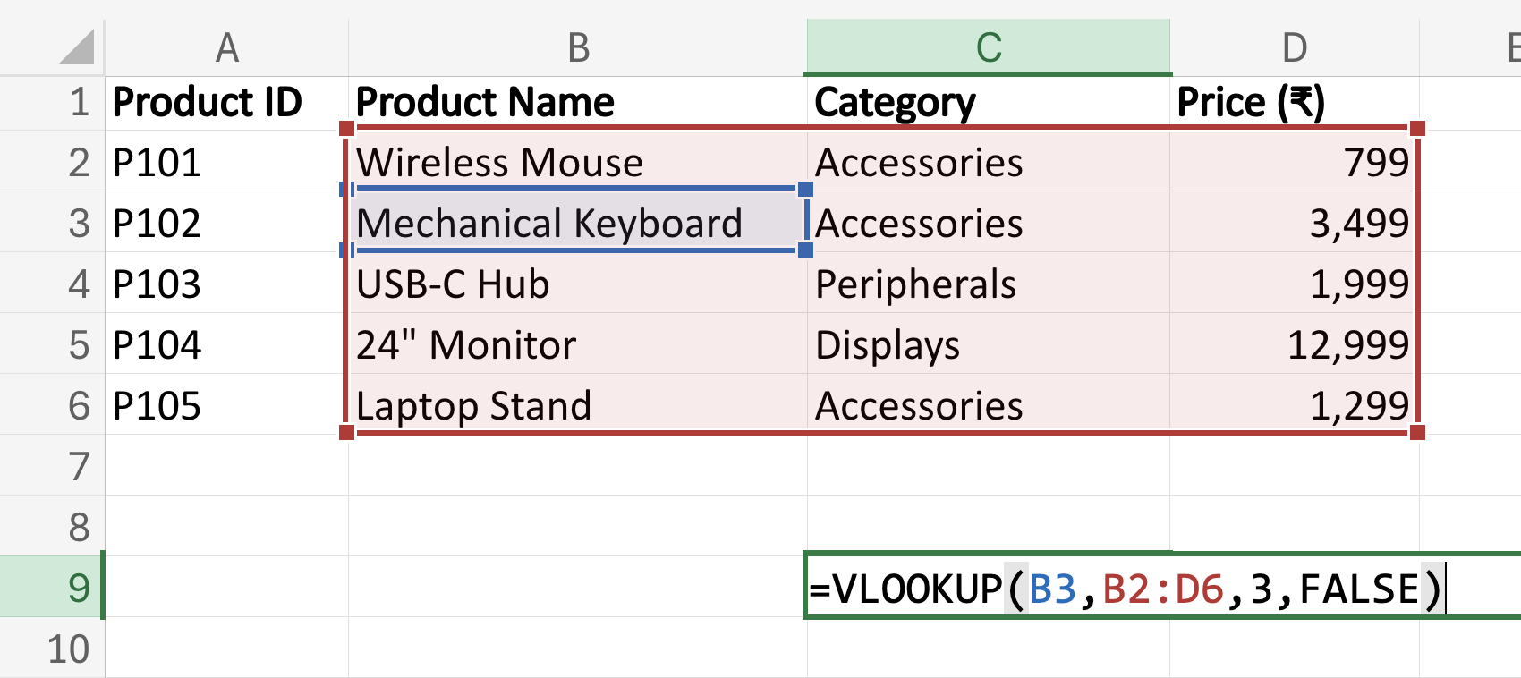
This may occasionally appear advanced at first, however don’t fear, we are going to stroll via this step-by-step.
Allow us to start with the terminology of the completely different components concerned right here, and the syntax that the formulation follows.
VLOOKUP Syntax
To make VLOOKUP work, you solely want 4 inputs – nothing extra. These are:
- Lookup worth: the worth you wish to seek for. In our instance, that is Mechanical Keyboard, since we want to discover its value.
- Desk vary: the place the information lives. In our case, that is full columns B to D.
Vital: the lookup worth have to be within the first column of this vary. - Column index quantity: which column incorporates the worth you need returned. (In case your vary is B:D, then B=1, C=2, D=3.)
- Match sort: That is non-obligatory typically. Listed below are the 2 varieties:
FALSE = precise match (most typical)
TRUE = approximate match (default should you go away it clean)
That’s it! These are the 4 inputs between you and by no means manually looking out a spreadsheet once more.
For successfully utilizing VLOOKUP, simply put all of it collectively as follows:
=VLOOKUP(lookup_value, table_range, column_index, FALSE/True)Forming the System
Now, allow us to evaluate this with the VLOOKUP formulation we got here up with for our instance above.
=VLOOKUP(B3,B2:D6,3,FALSE)- As you’ll be able to see within the desk, the time period “Mechanical Keyboard” is positioned at B3, and that’s our lookup_value. So we merely specify its place within the first occasion.
- Subsequent, we share the table_range, which in our case, is B2 to D6, as all the information is between these columns.
- Subsequent, we specify the column quantity from which we would like the information. Since it’s value, it’s below the ‘D’ column, which is the third column from our table_range (B=1, C=2, D=3). Therefore the three.
- Lastly, we select if we would like an actual match of the question, or simply an approximate match. Since we would like an actual match, we are going to use False.
And that’s it! Our VLOOKUP formulation is able to use. As you’ll be able to see within the desk, we have now accurately discovered our reply, i.e. a value of Rs 3,499 for the Mechanical Keyboard.
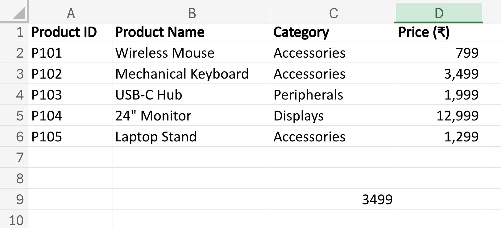
Simply to check should you’ve acquired it, strive framing the VLOOKUP formulation for locating the value of Laptop computer Stand. I’ll point out the proper reply on the finish of this text.
Assuming you’re clear with the essential ideas of VLOOKUP, let’s discover some particular eventualities by which it could require some tweaks.
Additionally learn: Finest Sources to be taught Microsoft Excel
Absolute References in VLOOKUP
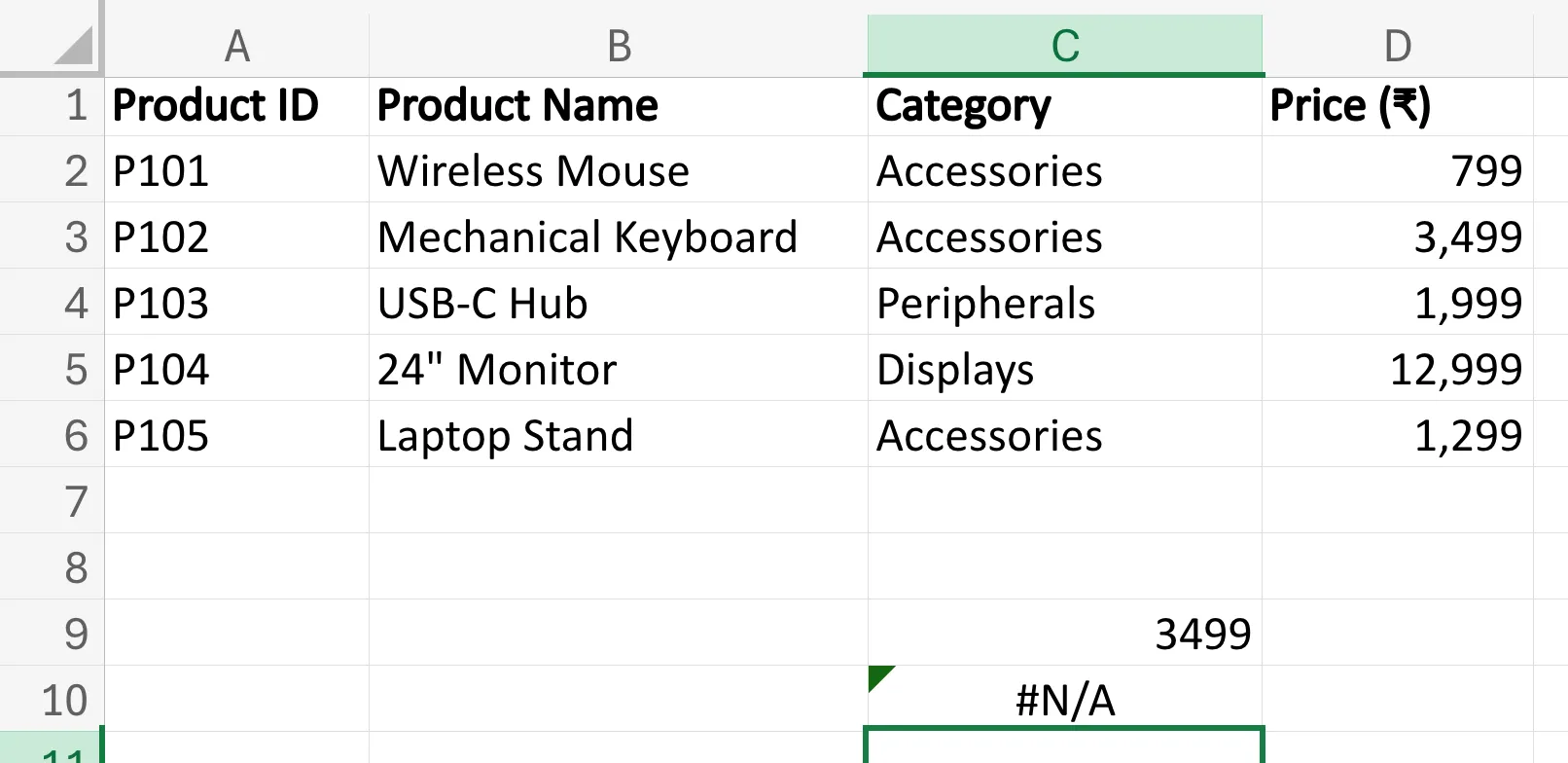
In the event you strive copying your VLOOKUP formulation down a column, you’ll face an surprising drawback: the formulation breaks. As an alternative of returning appropriate values, you may see errors or incorrect outcomes. This occurs as a result of Excel shifts the desk vary each time the VLOOKUP formulation is copied. This is called relative referencing.
By default, Excel assumes that references ought to transfer with the formulation. So in case your desk vary is B2:D6 and also you copy the formulation down one row, Excel adjusts it to B3:D7. The end result? Your lookup desk shifts… and your information could disappear.
That is the place absolute references save the day.
An absolute reference locks the desk vary so it doesn’t transfer when copied. You create it by including greenback indicators. So the common table_range turns into one thing like this:
B2:D6 → $B$2:$D$6You are able to do this immediately by deciding on the vary in your formulation and urgent F4.
When do you want this?
Think about you’re filling costs for 100 merchandise utilizing one grasp value desk. As an alternative of writing the formulation 100 instances, you write it as soon as and drag it down. With out absolute references, the lookup desk retains shifting, and the outcomes break. With $B$2:$D$6, the formulation all the time factors to the proper vary within the desk.
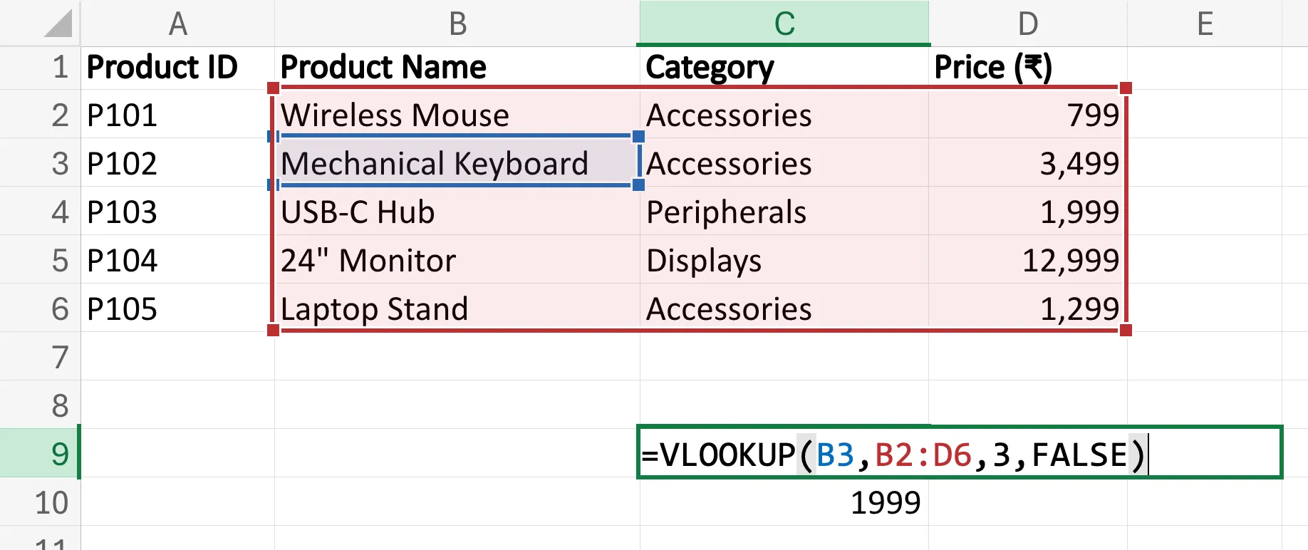
Checkout how the vary shifts within the screenshots beneath, once I copy/paste the VLOOKUP formulation only one row beneath. B2:D6 turns into B3:D7. Discover that on this case, the vary has solely skipped the primary row of knowledge, i.e. that of the Wi-fi Mouse on B2. So, if I ask for B2’s information now, VLOOKUP throws a #N/A error as seen beneath.
To keep away from this, we add absolute references within the table_range. The proper formulation then turns into:
=VLOOKUP(B3,$B$2:$D$6,3,FALSE)So, to summarise, absolute references guarantee your lookup desk stays mounted. With that, you’ll be able to scale your formulation confidently throughout a whole lot or hundreds of rows.
However wait, there may be one other approach to sort out relative referencing.
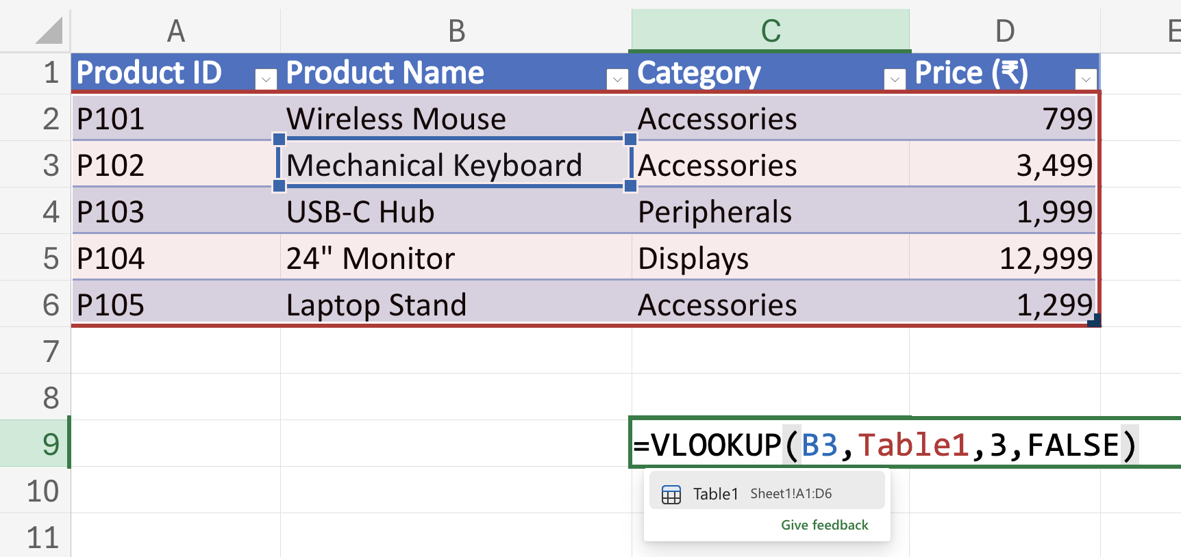
Utilizing Excel Tables with VLOOKUP
Whereas absolute references resolve the shifting-range drawback, there may be an excellent smarter approach to make your VLOOKUP formulation future-proof: Excel Tables.
Once you convert your information vary right into a desk, Excel robotically retains monitor of your complete dataset. The dataset stays intact even when new rows are added or previous ones are eliminated. This implies your VLOOKUP formulation continues to work with none guide updates.
Why is this convenient?
Think about that your warehouse checklist grows each week with new merchandise. In case your formulation references a set vary like $B$2:$D$6, you would want to replace it each time the desk expands. But when the information is saved in an Excel Desk, the formulation robotically contains the brand new entries.
Easy methods to convert information right into a desk
- Choose your dataset.
- Press Ctrl + T (or go to Insert → Desk).
- Verify that your desk has headers.
- Excel assigns a reputation comparable to Table1 (you’ll be able to rename it later).
- As an alternative of a cell vary, reference the desk title:
=VLOOKUP(B3,Table1,3,FALSE)
Now, each time new rows are added to the desk, the formulation nonetheless works completely.
When must you use Excel Tables?
- Rising datasets (gross sales logs, stock, buyer lists)
- Dashboards that replace repeatedly
- Reviews that require frequent information additions
- Collaborative spreadsheets the place the construction could change
Briefly, Excel Tables make your formulation smarter, extra dynamic, and maintenance-free — precisely what you need when working with real-world information.
Additionally learn: 50+ Excel Interview Inquiries to Ace Your Interview
Limitations of VLOOKUP
As highly effective as VLOOKUP is, it’s not good. Understanding its limitations will prevent hours of confusion later. Listed below are some:
- Lookup worth have to be within the first column:
VLOOKUP can solely search left → proper. If the worth you want lies to the left, the formulation received’t work. - Single match solely:
It returns the primary match it finds and never a number of outcomes. - Column numbers are static:
In the event you insert or rearrange columns, the column index can break and return incorrect outcomes. - Not preferrred for big datasets:
On very massive spreadsheets, VLOOKUP can gradual efficiency. - Approximate match pitfalls:
In the event you neglect to set FALSE, Excel defaults to an approximate match, which may produce unsuitable outcomes.
Due to these limitations, trendy Excel variations launched XLOOKUP, a extra versatile substitute that enables left lookups, dynamic columns, and extra correct matching.
That mentioned, VLOOKUP stays one of the broadly used and important capabilities you need to grasp. Listed below are some professional tricks to get probably the most out of it.
Professional Tricks to Grasp VLOOKUP
If you’d like VLOOKUP to work easily each time (and keep away from spreadsheet heartbreak), preserve these skilled suggestions in thoughts:
- All the time use FALSE for precise matches:
Actual match prevents incorrect outcomes, particularly when working with IDs, names, or codes. - Lock your desk vary with absolute references:
Press F4 to lock the vary ($B$2:$D$100) earlier than dragging the formulation down. - Use structured tables for dynamic information:
Convert ranges into Excel Tables (Ctrl + T) so your formulation auto-adjusts when information grows. Observe, use both this or absolute references, not each. - Double-check column index numbers:
A unsuitable index returns unsuitable information. And Excel received’t warn you. - Kind information when utilizing TRUE (approximate match):
Approximate match works accurately solely when the lookup column is sorted in ascending order. - Deal with errors gracefully with IFERROR:
The formulation =IFERROR(VLOOKUP(…),”Not Discovered”) prevents ugly #N/A errors. - Keep away from duplicates within the lookup column:
VLOOKUP returns the primary match solely. Duplicates can produce deceptive outcomes. - Use helper columns when wanted:
Mix fields (e.g., ID + Date) to create distinctive lookup keys.
Grasp these small habits, and VLOOKUP will really feel much less like a formulation and extra like a superpower.
Conclusion
VLOOKUP has earned its repute as considered one of Excel’s strongest and broadly used capabilities, and for good purpose. As we simply noticed via examples, it utterly eliminates tedious guide looking out. As an alternative, it brings a quick, dependable course of that may be scaled at will. Whether or not you’re employed in finance, operations, HR, gross sales, or analytics, mastering VLOOKUP can save hours of effort and considerably cut back errors.
Whereas newer capabilities like XLOOKUP supply added flexibility, VLOOKUP stays a foundational talent each Excel person ought to know. Study it as soon as, practise it with actual datasets, and also you’ll rapidly realise why it continues to energy spreadsheets throughout industries.
And sure! Right here is the proper formulation for the self-test train we did above:
=VLOOKUP(B6,B2:D6,3,False)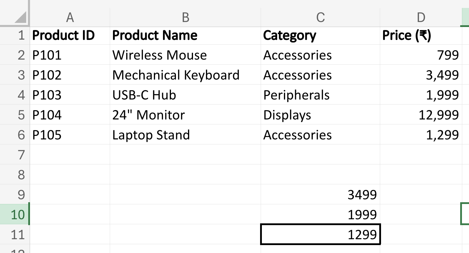
Login to proceed studying and luxuriate in expert-curated content material.